import numpy as np
import matplotlib.pyplot as plt

# 1. Define a "Ravine" Function: f(x,y) = 0.1x^2 + 2y^2
# It is much steeper in Y than in X.
def loss_function(x, y):
    return 0.1 * x**2 + 2 * y**2

def gradient(x, y):
    return np.array([0.2 * x, 4 * y])

# 2. Vanilla SGD Implementation
def run_sgd(start_pos, lr, steps):
    path = [start_pos]
    curr = np.array(start_pos)
    for _ in range(steps):
        grad = gradient(curr[0], curr[1])
        curr = curr - lr * grad
        path.append(curr)
return np.array(path)8 Optimization and Simulation in Machine Learning
8.1 Introduction
In the previous chapters, we treated optimization as a tool for decision-making, like finding the best shipping route or the optimal factory schedule. In these scenarios, the “model” was explicit. We knew the constraints, we knew the objective function, and we simply needed to find the variable values \(x\) that optimized the objective function. In Machine Learning (ML) and Artificial Intelligence (AI), the change the paradigm. We are no longer optimizing a specific decision, but rather learning a function that makes decisions.
From this perspective, ML is not magic, but simply optimization applied to function approximation. When we say a neural network “learns” to recognize a cat, we mean that an optimization algorithm has traversed a high-dimensional landscape and found a specific configuration of parameters (weights and biases) that minimizes the error between the network’s output and the label “cat.”
In general, we use a very specific notation when applying optimization to ML problems. We denote the input data as \(X\) and the output data (or labels) as \(y\). The model we are trying to learn is a function \(f(X; \theta)\), where \(\theta\) represents the parameters of the model (e.g., weights in a neural network). The goal of training the model is to find the optimal parameters \(\theta^*\) that minimize a loss function \(\mathcal{L}(y, f(X; \theta))\), which quantifies the difference between the predicted outputs and the true labels.
\[ \theta^* = \arg\min_{\theta}\frac{1}{n} \sum_{i=1}^n \mathcal{L}(y_i, f(x_i; \theta)) \]
However, not all problems come with a static dataset. In Reinforcement Learning (RL) or game playing (like Go or Chess), the “data” is generated dynamically by the agent’s interactions with the world. In this case, we often do not have an explicit formula for the objective function (e.g., “Win the game”) and we cannot calculate the gradient of “winning” directly. Instead, we must rely on simulation: We run the system forward in time (simulate a game, simulate a robot arm moving), observe the outcome, and use that empirical data to estimate the gradient or value.
Thus, modern AI is the marriage of optimization (improving parameters based on data) and simulation (generating data based on parameters).
In this chapter, we will explore how these concepts manifest in three distinct phases of the AI lifecycle:
Training: The process of optimizing model parameters using data samples. In this case, we rely on Stochastic Gradient Descent (SGD) and its adaptive variants (like Adam). These methods use the “noise” inherent in data sampling to navigate complex terrains where traditional Newton-type methods fail.
Planning: The process of simulating future states of the world to make better decisions in the present. Here, we will explore techniques like Monte Carlo Tree Search (MCTS) that allow agents to evaluate potential future actions by simulating their outcomes.
Interaction: The process of learning from real-time feedback as the agent interacts with its environment. This involves methods like Q-learning and Policy Gradients, which use simulations of the agent’s actions to improve its decision-making policy over time.
8.2 Optimization in Deep Learning
In Chapter 5, we established that convex problems are “easy” and non-convex problems are “hard.” Deep Learning places us firmly in the “hard” category. A modern neural network may have billions of parameters, and the relationship between these parameters and the loss function is highly non-linear. Despite this, we routinely train these models to near-perfect accuracy. How is this possible? The answer lies in the specific geometry of high-dimensional spaces and the specific properties of the algorithms we use.
8.2.1 The Loss Landscape in DL
For decades, researchers and practitioners in ML feared local minima: small valleys where the algorithm might get stuck, far higher than the global minimum. However, intuition derived from 2D or 3D surfaces is misleading in high dimensions. In 2D, a local minimum is a point where all directions lead uphill. In high dimensions, however, the number of directions increases dramatically. As a result, the probability of encountering a true local minimum (where all directions are uphill) decreases significantly. Instead, we often find “saddle points” or “flat regions” where some directions lead uphill while others lead downhill.
Probability theory tells us this is incredibly rare. In high-dimensional landscapes, most points where the gradient vanishes (\(\nabla \mathcal{L} = 0\)) are not minima, but saddle points. These are points that curve up in some directions but down in others. The main implication is that algorithms that rely solely on Newton’s method (using the Hessian) struggle here because the Hessian has both positive and negative eigenvalues. Gradient-based methods, however, can usually “slide off” the saddle point along the downward-sloping dimensions.
8.2.2 Backpropagation and Stochastic Gradient Descent
In general, to minimize the loss \(\mathcal{L}(\theta)\), we need the gradient \(\nabla \mathcal{L}(\theta)\). For a deep network, deriving this analytically is impossible. Instead, we use backpropagation. Put simply, backpropagation is simply the recursive application of the familiar chain rule of calculus on a computational graph. It involves two passes through the network: a forward pass to compute the output and loss, and a backward pass to compute the gradients of the loss with respect to each parameter. Modern Deep Learning frameworks like PyTorch utilize Automatic Differentiation (AutoDiff): only the forward pass is needed, and the software automatically constructs the graph to compute the backward pass.
Standard Gradient Descent (Batch GD) computes the gradient over the entire dataset before taking a step.
\[ \theta_{k+1} = \theta_k - \eta \frac{1}{n} \sum_{i=1}^n \nabla \mathcal{L}_i(\theta_k) \]
where \(\mathcal{L}_i\) is the loss for the \(i\)-th data point, and \(\eta\) is the learning rate. However, for large datasets, this is computationally expensive. Instead, we use Stochastic Gradient Descent (SGD), which approximates the gradient using a small batch of data points.
\[ \theta_{k+1} = \theta_k - \eta \frac{1}{m} \sum_{i=1}^m \nabla \mathcal{L}_{j_i}(\theta_k) \]
where \(m\) is the batch size, and \(j_i\) are randomly selected indices from the dataset. This introduces noise into the gradient estimate, which can help the optimization process escape saddle points and explore the loss landscape more effectively.
The landscape of a neural network often features ravines: areas that are steep in one dimension but flat in another. Standard SGD tends to oscillate wildly across the steep slopes while making slow progress along the flat bottom. To fix this, we use algorithms that adapt the update step for each parameter individually.
Momentum
Momentum is a technique that helps accelerate SGD in the relevant direction and dampens oscillations. It does this by maintaining a velocity vector that accumulates the gradients over time. \[ v_{k+1} = \beta v_k + (1 - \beta) \nabla \mathcal{L}(\theta_k) \] \[ \theta_{k+1} = \theta_k - \eta v_{k+1} \]
Where \(\beta\) is a new hyperparameter that we call momentum and takes values between 0 and 1. In practice, this parameter is usually set to around 0.9.
Adam
The other idea is called Adaptive Moment Estimation (Adam). Adam maintains two moving averages: one for the gradients (first moment) and one for the squared gradients (second moment).
\[ m_{k+1} = \beta_1 m_k + (1 - \beta_1) \nabla \mathcal{L}(\theta_k) \] \[ v_{k+1} = \beta_2 v_k + (1 - \beta_2) (\nabla \mathcal{L}(\theta_k))^2 \]
\[ \theta_{k+1} = \theta_k - \eta \frac{m_{k+1}}{\sqrt{v_{k+1}} + \epsilon} \]
Where \(\beta_1\) and \(\beta_2\) are hyperparameters that control the decay rates of these moving averages, typically set to 0.9 and 0.999, respectively. The small constant \(\epsilon\) is added to prevent division by zero.
Let’s take a look at a scratch implementation of Vanilla SGD and Adam in Python:
Now we implement Adam:
# 3. Adam Implementation (Simplified)
def run_adam(start_pos, lr, steps, beta1=0.9, beta2=0.999, epsilon=1e-8):
    path = [start_pos]
    curr = np.array(start_pos)
    m = np.zeros(2) # First moment (Momentum)
    v = np.zeros(2) # Second moment (Variance)

    for t in range(1, steps + 1):
        grad = gradient(curr[0], curr[1])

        # Update moments
        m = beta1 * m + (1 - beta1) * grad
        v = beta2 * v + (1 - beta2) * (grad**2)

        # Bias correction (important for early steps)
        m_hat = m / (1 - beta1**t)
        v_hat = v / (1 - beta2**t)

        # Update parameters
        curr = curr - lr * m_hat / (np.sqrt(v_hat) + epsilon)
        path.append(curr)
    return np.array(path)
In this implementation, we have added a bias correction step to the moment estimates. This is crucial, especially in the early stages of training, to ensure that the estimates are unbiased. Now we visualize the results:
start = [-10.0, -2.0] # Start far away
steps = 50
lr = 0.1

path_sgd = run_sgd(start, lr, steps)
path_adam = run_adam(start, lr, steps)

# Create contour map
X, Y = np.meshgrid(np.linspace(-12, 2, 100), np.linspace(-4, 4, 100))
Z = loss_function(X, Y)
plt.contour(X, Y, Z, levels=20, cmap='gray', alpha=0.4)

plt.plot(path_sgd[:,0], path_sgd[:,1], 'o-', label='SGD', color='red')
plt.plot(path_adam[:,0], path_adam[:,1], 'o-', label='Adam', color='blue')

plt.title("Optimization Trajectories: Ravine Problem")
plt.legend()
plt.grid(True)
plt.show()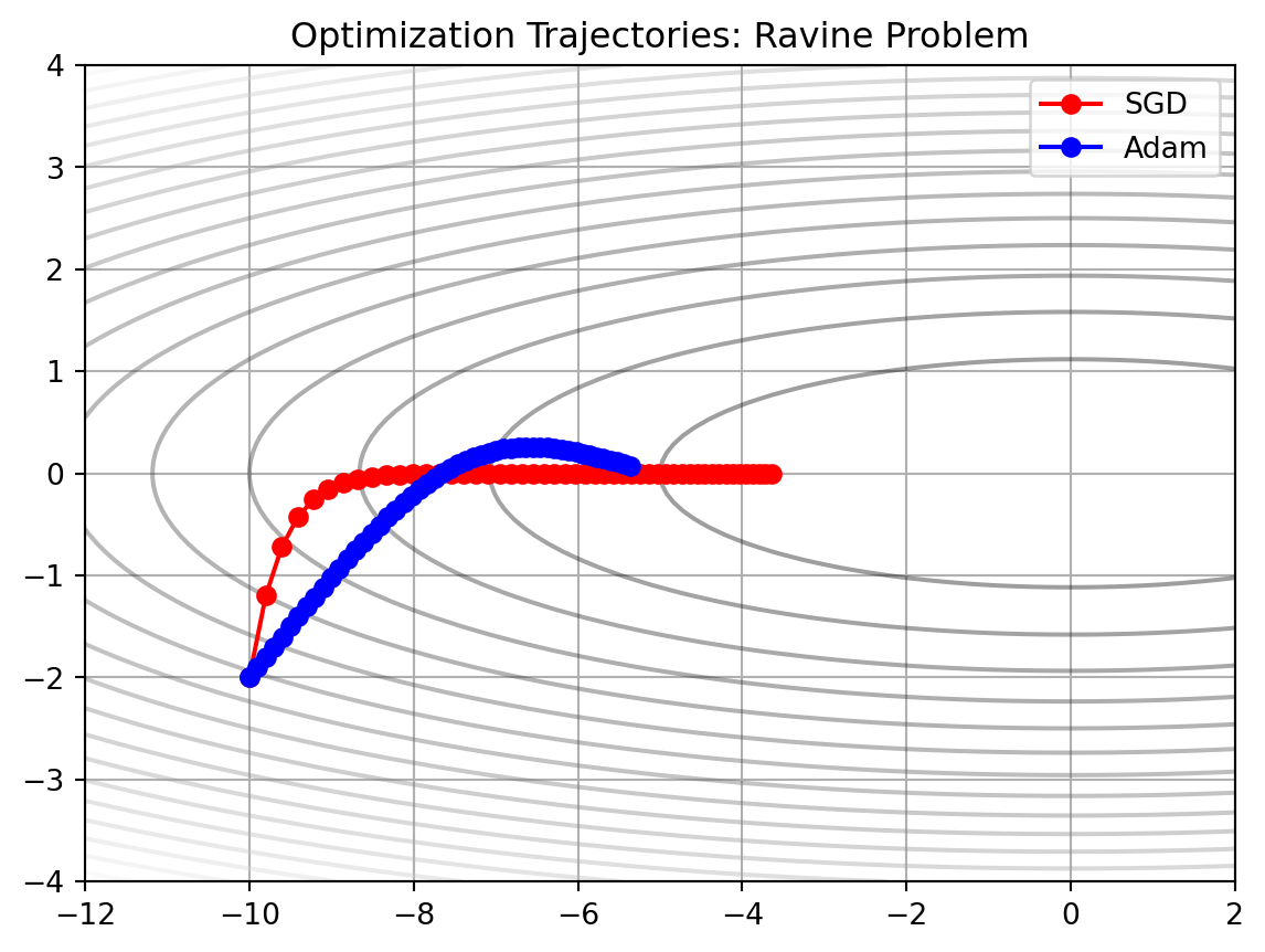
In this graph, SGD oscillates vertically (along the steep \(Y\)-axis) while making very slow progress horizontally (along the flat \(X\)-axis). It struggles to find the right step size for both dimensions simultaneously. In contrast, Adam quickly adapts. It dampens the step size in \(Y\) (high gradient) and boosts the step size in \(X\) (low gradient), shooting directly toward the center minimum. This behavior is why Adam is the standard for training deep networks.
8.3 Monte Carlo Tree Search
In the previous section, we discussed optimizing a static function (the loss of a neural network). Now, we turn to planning: deciding what action to take in a complex, sequential environment, such as playing chess, routing a fleet of drones, or folding a protein. Historically, AI planning relied on Minimax search with heuristic evaluation functions. To know if a chess board state was “good,” a human expert had to write a scoring function (e.g. \(10\times\) if queens are on the board + \(5\times\) number of rooks, etc). However, for complex situations like playing a game of Go or folding proteins, writing a good evaluation function gets too challenging.
This is where Monte Carlo simulation comes in. Instead of asking an expert “Is this state good?”, we ask the computer to play it out. We simulate thousands of random games starting from the current state. If we win 80% of those random games, the state is likely “good”. If we win only 10%, it is likely “bad”.
In the planning context, we call this a rollout:
- Start at initial state \(S_t\).
- Select actions \(a_t, a_{t+1}, \dots\) until a terminal state (Win/Loss) is reached.
- Record the result: +1 if win, 0 if loss.
- Repeat \(N\) times.
- Estimate the value of \(S_t\) as \(\text{Total Wins}/N\).
However, classical Monte Carlo Simulation has a flaw: it wastes computational resources exploring obviously bad moves. If you hang your queen in chess, you don’t need 1,000 simulations to know it’s a bad idea; you need 1.
Monte Carlo Tree Search (MCTS) solves this by building a search tree asymmetrically. It uses the results of previous simulations to guide future simulations toward more promising parts of the tree, trying to balance exploitation (by focusing on moves with a high win rate) and exploration (by simulting moves that have few visits, just in case they turn out to be good).
MCTS runs a loop of four steps as many times as the computing budget allows:
- Selection: We start at the root and traverse down the tree by selecting child nodes. At each step, we choose the child that maximizes the Upper Confidence Bound (UCT) formula (see Equation 8.1), stopping when a node that has not been fully expanded is reached.
- Expansion: Add one or more child nodes to the tree (representing available moves from that state).
- Simulation: From the new child node, play a random game to the end (rollout).
- Backpropagation: Take the result of the simulation (Win/Loss) and walk back up the tree to the root, updating the statistics (wins and visits) for every node on the path.
The UCB formula is given by:
\[ UCT_i = \frac{w_i}{n_i}+c\sqrt{\frac{\ln N}{n_i}} \tag{8.1}\]
where \(w_i\) denotes the number of wins for child node \(i\), \(n_i\) is the number of times that node \(i\) has been visited, \(N\) is the total number of visits to the parent node, and \(c\) is an exploration constant (typically \(c=\sqrt{2}\)).
We can interpret \(w_i/n_i\) as the average win rate, which encourages exploitation. The other term (\(\sqrt{\dots}\)) is an uncertainty “bonus”: if a node is rarely visited (\(n_i\) is small), this term becomes larger, which encourages exploration. As we proceed and visit more nodes, \(n_i\) becomes larger and the search concentrates more on the exploitation term.
MCTS allows an agent to plan in environments where it has no prior knowledge. It does not need to know strategy; it discovers strategy by simulating thousands of futures. E.g. in AlphaZero, this simulation data is used to train a Neural Network, which in turn guides the MCTS Selection phase, creating a cycle of self-improvement.
We now take a look at a sample generic implementation of MCTS. We start by defining a node in the search tree.
import math
import random
import copy

class MCTSNode:
    def __init__(self, state, parent=None):
        self.state = state
        self.parent = parent
        self.children = []
        self.wins = 0
        self.visits = 0
        self.untried_moves = state.get_legal_moves()

    def uct_select_child(self, c=1.41):
        # Sort children by UCT formula
        s = sorted(self.children, key=lambda child:
            (child.wins / child.visits) + c * math.sqrt(math.log(self.visits) / child.visits))
        return s[-1] # Return the best
An MCTS node tracks the number of wins, visits, the problem-dependent state, and the number of untried moves. Additionally, is provides a method for selectin the best child according to Equation 8.1.
The main MCTS algorithm with the four phases mentioned before can be implemented as follows:
def run_mcts(root_state, iterations=1000):
    root_node = MCTSNode(root_state)

    for _ in range(iterations):
        node = root_node
        state = copy.deepcopy(root_state)

        # Phase 1: Selection
        # Go down the tree until we hit a node with untried moves or a terminal state
        while node.untried_moves == [] and node.children != []:
            node = node.uct_select_child()
            state = state.make_move(node.move_from_parent) # Need to track moves in real impl

        # Phase 2: Expansion
        # If we can expand, add one child
        if node.untried_moves != []:
            m = random.choice(node.untried_moves)
            state = state.make_move(m)
            node = node.add_child(m, state) # Pseudo-code: create child logic

        # Phase 3: Simulation (Rollout)
        # Play randomly until end
        while state.check_winner() is None:
            state = state.make_move(random.choice(state.get_legal_moves()))

        # Phase 4: Backpropagation
        # Update stats up the tree
        winner = state.check_winner()
        while node is not None:
            node.visits += 1
            # If the player at this node won, increment wins
            # (Note: In real MCTS, we must be careful about whose turn it is)
            if winner == node.state.player_who_just_moved:
                node.wins += 1
            node = node.parent

    # Return the move with the most visits (most robust)
    return sorted(root_node.children, key=lambda c: c.visits)[-1].move_from_parent
The make_move and check_winner methods would need to be implemented for the specific problem at hand.
8.4 Reinforcement Learning
We now very briefly introduce Reinforcement Learning and frame it as an optimization method. In Supervised Learning, the optimization target is static (minimize the training error on a fixed dataset). In constrast, in Reinforcement Learning (RL), the target is dynamic. We are optimizing a sequence of decisions over time, where a decision made now determines the data we see later. The mathematical foundation of RL is based on the concept of a Markov Decision Process (MDP), as we will see next.
8.4.1 Markov Decision Processes
The mathematical formalism of Markov Decision Processes underpins how optimization in RL is framed. We start with the following elements:
- State Space \(S\): The set of all possible configurations (e.g. in chess, the set of all legal chess board states).
- Action Space \(A:\) The set of all possible actions that an agent can take (e.g. the set of all legal moves in a game).
- Transition Probabilities \(P\): The rules for transitioning from one state to another. In general, this is represented by a probability distribution \(P(s'|s,a)\) of states conditional on the previous state \(s\) and the action taken \(a\).
- Reward Function \(R\): The immediate reward \(R(s,a)\) the agent collects on state \(s\) after performing action \(a\).
- Discount Factor \(\gamma\): A number between 0 and 1 that weighs immediate rewards against future rewards.
Our goal is to find a policy \(\pi(a|s)\) that maps states to actions that maximizes the expected discounted return:
\[ J(\pi)=E\left[\sum_{t=0}^\infty \gamma^t r_t\right] \]
This can be framed as a constrained optimization problem: maximize \(J\) subject to the constraints of the environment dynamics.
8.4.2 Value-based Methods
One approach to solving this is to ignore the policy initially and focus on maximizing a notion of value. If we knew exactly how good every state was (the “Value Function”), the optimal policy would simply be “move to the state with the highest value”. We can define the value of a state-action pair \(Q(s,a)\) recursively as follows (Bellman equation):
\[ Q(s,a)=R(s,a)+\gamma \max_{a'} Q(s',a') \]
which means that the value of an action is the immediate reward plus the best possible future value.
We can approximate the true \(Q(s,a)\) using a deep neural network \(Q(s,a;\theta)\), in what we call Deep Q-Learning (DQN). We can train this network by minimizing the mean squared error (also called Bellman error, or Temporal Differences error):
\[ \mathcal{L}(\theta)=E\left[ \left( r+\gamma\max_{a'}Q(s',a';\theta_{target})-Q(s,a;\theta) \right)^2\right] \tag{8.2}\]
In this function, we measure the difference between the prediction from the neural network \(Q(s,a;\theta)\) and the current estimate of the target term:
\[ y=r+\gamma\max_{a'}Q(s',a';\theta_{target}) \]
In this target, \(r\) is the reward which was actually experienced by the agent. However, the second term is just the current best estimate on how much reward it is expected in the future. In summary, we are using the network’s own prediction of the future to train its prediction of the present. This is sometimes referred to as bootstrapping.
This method is also referred to as an instance of model-free RL. In this case, we do not have a model of how the physical world works, but we can simulate several actions of the agent to obtain tuples \((s,a,r,s',\text{done})\) that we store in a so-called replay buffer. Once we have this buffer, we can feed these data on a training episode and use Equation 8.2 to update the weights \(\theta\) of the neural network. Note that in this equation, we have two sets of weights \(\theta_{target}\) and \(\theta\). The weights which are currently being optimized are \(\theta\), while \(\theta_{target}\) is a frozen copy used for calculating the \(\max\) term. This is done in order to prevent the training process from “chasing its own tail”, as otherwise the network predictions would change with each gradient update.
8.4.3 Policy-Based Methods
Alternatively, we can try to optimize the policy \(\pi_{\theta}(a|s)\) directly instead of the value function \(Q(s,a)\). However, because the environment is usually a “black-box” or a discrete simulation, we cannot calculate the gradient \(\nabla_\theta J(\theta)\) directly.
\[ \nabla_\theta J(\theta)=\nabla_\theta E_{\tau\sim\pi}\left[ R(\tau) \right]=\nabla_\theta \int P(\tau|\theta)R(\tau)d\tau \]
The main difficulty with this calculation is that we cannot differentiate this integral to obtain the gradient. However, we can use a property of the derivative of a logarithm (the log-derivative trick) to transform it into the integral of a derivative instead.
\[ \frac{d}{dx}\ln f(x)=\frac{f'(x)}{f(x)} \Rightarrow f'(x)=f(x)\frac{d}{dx}\ln f(x) \] \[ \nabla_\theta P(\tau|\theta)=P(\tau|\theta)\cdot\nabla_\theta \ln P(\tau|\theta) \]
which converts the previous integral in:
\[ \nabla_\theta J(\theta)=\int P(\tau|\theta)\nabla_\theta \ln P(\tau|\theta)\cdot R(\tau)d\tau=E_{\tau\sim\pi}\left[ \nabla_\theta\ln P(\theta|\phi)\cdot R(\theta) \right] \]
Using the estimates that we have, we can approximate the gradient of the expected reward as follows:
\[ \nabla_\theta J(\theta)\approx E\left[ \sum_{t=0}^T \nabla_\theta \ln \pi_\theta(a_t|s_t)\cdot G_t \right] \]
where:
- \(G_t\) is the total return obtained from time \(t\) onwards. \[ G_t=r_t+\gamma r_{t+1}+\gamma^2 r_{t+2}+\dots \]
- \(\nabla \ln \pi(a|s)\) tells us how to change \(\theta\) to make action \(a\) more or less probable.
In other words, if \(G_t\) is positive (good outcome), we move \(\theta\) to increase the probability of the action. Otherwise, if \(G_t\) is negative (bad outcome), we move \(\theta\) to decrease that probability. This is known as the REINFORCE algorithm, and it’s another instance of model-free RL.
8.4.4 Model-Based Reinforcement Learning
The methods mentioned above are model-free: they learn purely from experience without having any knowledge about how those experiences are formed. By contrast, in model-based RL our goal is to learn a model of the world, i.e. the transition function \(P(s'|s,a)\). Once that the agent has learnt this model, we can use techniques like DQL more efficiently by, for instance, simulating training data and using real and synthetic data to train the agent.
8.5 Case Study: AlphaZero
In 2017, DeepMind introduced AlphaZero, a system that mastered the games of Chess, Shogi, and Go. Unlike its predecessor AlphaGo (which learned from human games) or Deep Blue (which relied on handcrafted heuristics), AlphaZero started from scratch. It knew only the rules of the game. As we will see next, AlphaZero as a case study unifies the themes outlined in this chapter: simulation, function approximation, and optimization.
At the heart of AlphaZero is a single Deep Residual Network (ResNet), parameterized by weights \(\theta\), which takes board data \(s\) as input. Unlike traditional engines that have separate modules for strategy and evaluation, AlphaZero uses a single network with two output “heads”:
- The Policy Head: Outputs a probability distribution \(p(a|s)\) over all legal moves. This represents the “intuition” of the agent.
- The Value Head: Outputs a single scalar \(v(s)\in[-1,1]\) as the expected outcome from state \(s\) (+1 for win, -1 for loss). This represents the “judgement” of the agent.
Now the critical insight of AlphaZero is how it uses MCTS. In traditional AI, search is used only at runtime to play the game. In AlphaZero, search is used during training to generate the data. AlphaZero uses a neural network to guide the MCTS selection process. For this, we need a modified UCT formula to include the network’s prior probability \(P(s,a)\):
\[ UCT(s,a)=Q(s,a)+c\cdot P(s,a)\cdot\frac{\sqrt{N(s)}}{1+N(s,a)} \tag{8.3}\]
where:
- \(Q(s,a)\) is the average value of all simulations that passed through this specific state-action pair. It is calculated as the average of the Value Head outputs \(v\) of the leaf nodes reached by this branch. Its role is exploitation by representing the empirical evidence gathered so far: “Does this move actually lead to a win?”.
- \(P(s,a)\) is the probability assigned to action \(a\) by the Policy Head when it first evaluated state \(s\). It represents the agent’s intuition: “Does this move look like a good move?”.
- \(N(s)\) is the parent visit count, or total number of times the parent node (state \(s\)) has been visited.
- \(N(s,a)\) is the child visit count, or number of times a specific action \(a\) has been selected from state \(s\). Since this appears in the denominator, as we visit a specific move more often, this term grows, reducing the influence of the exploration bonus.
- \(c\) is an exploration constant, a hyperparameter that determines how much we rely on the prior \(P(s,a)\) versus the empirical value \(Q(s,a)\).
After running a large number of simulations for a single move, the MCTS produces a visit count distribution. We normalize these visit counts to create a new probability distribution \(\pi\). This distribution represents a stronger policy than the raw network output \(p_\theta(s)\), since the search process has “purified” the intuition (the prior).
8.5.1 The Training Process
The training process is a continuous loop of self-improvement.
- Self-Play (Simulation): The agent plays games against itself. At every step, it runs MCTS to generate the improved policy \(\pi\) and selects a move. It plays until the game ends, producing a final outcome \(z\in\{-1,+1\}\).
- Data Generation: For every position in the game, we store a training example \((s,\pi,z)\), where \(s\) represents the board state, \(\pi\) is what MCTS said was the best action and \(z\) represents the actual result (who won the game).
- Optimization: We optimize the network parameters \(\theta\) to minimize the error between its predictions and the MCTS data.
\[ \mathcal{L}(\theta)=\underbrace{(z-v_\theta(s))^2}_{\text{Value loss}} - \underbrace{\pi^T\log p_\theta(s)}_{\text{Policy loss}} + \underbrace{c\lVert \theta \rVert^2}_{\text{Regularization}} \]
where the value loss is the MSE of the network predictions regarding the actual winner \(z\) and the policy loss is the cross-entropy of the network trying to mimic the MCTS search probabilities (\(\pi\)).
8.5.2 Simulation becomes Intuition
AlphaZero then learns the following way: Initially, the network is random and MCTS relies heavily on random rollouts. However, over time MCTS starts discovering winning strategies and the optimization steps forces the neural network to learn those strategies. As the neural network improves, its predictions (\(p\) and \(v\)) become more accurate, which improves MCTS (since \(p\) guides the search) to look deeper and find more subtle strategies.
This is the essence of optimization and simulation in ML: We use computationally expensive simulation (MCTS) to generate high-quality ground truth data, and then use optimization (SGD) to distill that complex simulation into a fast, efficient function approximator (the neural network). The result is an agent that possesses the “instinct” of a grandmaster.
8.6 Summary
In this chapter, we crossed the threshold from classical optimization—where the goal is to find the best value for a variable—to Machine Learning, where the goal is to find the best function to approximate reality.
We began by framing Deep Learning as a high-dimensional, non-convex optimization problem. We saw that the primary obstacles in training neural networks are not local minima, but saddle points and ill-conditioned curvature (ravines). We explored how Stochastic Gradient Descent (SGD) utilizes the noise of mini-batches to escape these traps, and how adaptive methods like Adam approximate the diagonal of the Hessian to normalize step sizes, allowing for efficient training on rugged landscapes.
Next, we moved from static functions to dynamic planning using Monte Carlo Tree Search (MCTS). We learned that when an objective function is too complex to define analytically (like the strategy of Go), we can estimate it through Simulation. By balancing exploration and exploitation via the UCT formula, MCTS builds an asymmetric search tree that focuses computational resources on the most promising futures.
Finally, we unified these concepts under Reinforcement Learning (RL). We framed sequential decision-making as an optimization problem over time, solving it either by approximating the value function (Deep Q-Learning) or by optimizing the policy directly (REINFORCE). We concluded with the case study of AlphaZero, which demonstrated that state-of-the-art AI is not magic, but a virtuous cycle: Simulation (MCTS) generates data to train a Function Approximator (Neural Network), which in turn guides the simulation to be more efficient.
8.7 Exercises
Consider the 2D “Rosenbrock-like” function, which features a narrow, curved valley: \[ f(x,y)=(1-x)^2+100(y-x^2)^2 \] Implement the gradient \(\nabla f(x,y)\) as a Python function and then Vanilla SGD with a fixed learning rate of \(\eta=0.001\). Implement the Adam optimizer with \(\eta=0.1\), \(\beta_1=0.9\) and \(\beta_2=0.999\). Start both optimizers at \((-1.5, -1.0)\) and run for 200 steps. Visualize the trajectory of both optimizers on a contour plot and explain why SGD oscillates or gets stuck, while Adam follows the valley floor.
Consider a node \(S\) in a MCTS game tree. The node has been visited \(N=50\) times and has two child nodes \(A\) and \(B\). The statistics for the child nodes are as follows:
- Child \(A\): Wins = 12, Visits = 20.
- Child \(B\): Wins = 18, Visits = 30.
The exploration constant is \(c=\sqrt{2}\). Calculate the UCT value for the child nodes \(A\) and \(B\) and select the next node according to the result. Suppose we visit the parent \(S\) an additional 50 times (\(N=100\)), but we never visit child \(A\) again. Calculate the new UCT value for \(A\).
Assume an agent in a Gridworld at state \(s=(1,1)\). When it takes the action “Right”, moving to state \(s'=(1,2)\), it receives a reward \(r=-1\). Let the discount factor be \(\gamma=0.9\) and the learning rate \(\alpha=0.1\). The \(Q\)-values for the next state are:
- \(Q(s', \text{Up})=-2.0\).
- \(Q(s', \text{Right})=-1.0\).
- \(Q(s', \text{Down})=-4.0\).
- \(Q(s', \text{Left})=-3.0\).
Calculate the temporal differences error and update the \(Q\)-value \(Q((1,1), \text{Right})\) using the standard Q-Learning update rule.
In the context of AlphaZero, let \((s,a)\) be state-move pair with a low probability \(P(s,a)\). Imagine that this move is a forced checkmate sequence (win). Taking Equation 8.3 into account, explain how MCTS can eventually discover and select this move despite the network’s initial bias against it. Which term in the formula drives this correction?